11. Strain and compatibility
After completing this chapter, you should be able to:
- Describe deformation with the displacement field \(\vec{u}(\vec{r})\)
- Decompose the displacement gradient into strain (symmetric) and rotation (antisymmetric) parts
- Interpret the components of the strain tensor geometrically
- Check whether a strain field is compatible, i.e. derives from a continuous displacement field
In Chapter 9, we introduced the stress tensor and derived the equilibrium equations that govern forces inside a solid body. However, equilibrium alone does not tell us how a body deforms under load. To connect forces to deformation, we need to introduce the concepts of displacement and strain. Together with Hooke’s law (which we will discuss in Chapter 13), these concepts complete the set of equations needed to solve problems in linear elasticity.
Displacement
When a solid body is subjected to external forces, its material points move from their original positions to new positions. The displacement field \(\vec{u}(\vec{r})\) describes this motion mathematically. Given a material point that was originally located at position \(\vec{r}\) in the undeformed (reference) configuration, its new position after deformation is \[\vec{r}' = \vec{r} + \vec{u}(\vec{r}).\] The displacement \(\vec{u}\) is therefore the vector pointing from the original position to the deformed position. Note that the displacement field is defined as a function of the reference position \(\vec{r}\), not the deformed position \(\vec{r}'\). This choice, called the Lagrangian or material description, is standard in solid mechanics because it allows us to track what happens to specific material points.
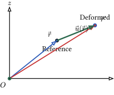
The displacement field \(\vec{u}(\vec{r})\) has three components in three-dimensional space, \[\vec{u} = \begin{pmatrix} u_x(x,y,z) \\ u_y(x,y,z) \\ u_z(x,y,z) \end{pmatrix},\] where each component can vary with position throughout the body. A uniform displacement \(\vec{u} = \text{const}\) corresponds to a rigid-body translation: all points move by the same amount, and the body does not deform. More interesting cases arise when the displacement varies from point to point, which leads to the concept of strain.
From displacement to strain
Why the displacement gradient matters
To understand deformation, we need to examine how displacement varies spatially. Consider two neighboring material points, one at position \(\vec{r}\) and another at \(\vec{r} + \mathrm{d}\vec{r}\), where \(\mathrm{d}\vec{r}\) is an infinitesimally small vector connecting them. In the reference configuration, these points are separated by the distance \(|\mathrm{d}\vec{r}|\). After deformation, the first point moves to \(\vec{r} + \vec{u}(\vec{r})\) and the second to \(\vec{r} + \mathrm{d}\vec{r} + \vec{u}(\vec{r} + \mathrm{d}\vec{r})\). The vector connecting them in the deformed configuration is \[\mathrm{d}\vec{r}' = \mathrm{d}\vec{r} + \vec{u}(\vec{r} + \mathrm{d}\vec{r}) - \vec{u}(\vec{r}).\]
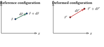
Using a Taylor expansion and keeping only first-order terms (which is valid for small displacements), we obtain \[\vec{u}(\vec{r} + \mathrm{d}\vec{r}) - \vec{u}(\vec{r}) \approx (\nabla \vec{u}) \cdot \mathrm{d}\vec{r},\] where \(\nabla \vec{u}\) is the displacement gradient tensor. This second-rank tensor contains all the information about how the displacement field varies in space. Its components are the partial derivatives \[[\nabla \vec{u}]_{ij} = \frac{\partial u_i}{\partial r_j} \equiv u_{i,j},\] where we have introduced the comma notation \(u_{i,j}\) as shorthand for partial differentiation. Written as a matrix, the displacement gradient is \[\nabla \vec{u} = \begin{pmatrix} \frac{\partial u_x}{\partial x} & \frac{\partial u_x}{\partial y} & \frac{\partial u_x}{\partial z} \\[6pt] \frac{\partial u_y}{\partial x} & \frac{\partial u_y}{\partial y} & \frac{\partial u_y}{\partial z} \\[6pt] \frac{\partial u_z}{\partial x} & \frac{\partial u_z}{\partial y} & \frac{\partial u_z}{\partial z} \end{pmatrix}.\]
It is important to distinguish the displacement gradient \(\nabla \vec{u}\) (a tensor) from the divergence \(\nabla \cdot \vec{u}\) (a scalar). The gradient tells us how the vector field changes in different directions, while the divergence only tells us whether the field is expanding or contracting at a point.
Decomposing the displacement gradient
The displacement gradient \(\nabla \vec{u}\) is a general second-rank tensor that need not be symmetric. Any such tensor can be uniquely decomposed into a symmetric part and an antisymmetric part, \[\nabla \vec{u} = \underbrace{\frac{1}{2}\left(\nabla \vec{u} + (\nabla \vec{u})^T\right)}_{\underline{\varepsilon}} + \underbrace{\frac{1}{2}\left(\nabla \vec{u} - (\nabla \vec{u})^T\right)}_{\underline{\omega}}.\] The symmetric part \(\underline{\varepsilon}\) is called the strain tensor, and the antisymmetric part \(\underline{\omega}\) is called the rotation tensor. This decomposition has profound physical significance: the strain tensor describes pure deformation (changes in shape and size), while the rotation tensor describes rigid-body rotation (changes in orientation without deformation).
The strain tensor
Definition and components
The strain tensor is defined as the symmetric part of the displacement gradient, \[\begin{equation} \label{eq:straingradient} \underline{\varepsilon}(\vec{r}) = \frac{1}{2}\left(\nabla \vec{u} + (\nabla \vec{u})^T\right). \end{equation}\] In component notation, the strain tensor elements are \[\begin{equation} \label{eq:straingradientcomp} \varepsilon_{ij} = \frac{1}{2}(u_{i,j} + u_{j,i}) = \frac{1}{2}\left(\frac{\partial u_i}{\partial r_j} + \frac{\partial u_j}{\partial r_i}\right). \end{equation}\] Note that this expression does not contain an implicit sum because there are no repeated indices. The symmetrization ensures that \(\varepsilon_{ij} = \varepsilon_{ji}\), so the strain tensor has only six independent components rather than nine.
Written explicitly as a matrix, the strain tensor is \[\underline{\varepsilon} = \begin{pmatrix} \varepsilon_{xx} & \varepsilon_{xy} & \varepsilon_{xz} \\ \varepsilon_{xy} & \varepsilon_{yy} & \varepsilon_{yz} \\ \varepsilon_{xz} & \varepsilon_{yz} & \varepsilon_{zz} \end{pmatrix}\] where the diagonal components are \[\begin{align} \varepsilon_{xx} &= \frac{\partial u_x}{\partial x}, \quad \varepsilon_{yy} = \frac{\partial u_y}{\partial y}, \quad \varepsilon_{zz} = \frac{\partial u_z}{\partial z}, \end{align}\] and the off-diagonal components are \[\begin{align} \varepsilon_{xy} &= \frac{1}{2}\left(\frac{\partial u_x}{\partial y} + \frac{\partial u_y}{\partial x}\right), \\ \varepsilon_{xz} &= \frac{1}{2}\left(\frac{\partial u_x}{\partial z} + \frac{\partial u_z}{\partial x}\right), \\ \varepsilon_{yz} &= \frac{1}{2}\left(\frac{\partial u_y}{\partial z} + \frac{\partial u_z}{\partial y}\right). \end{align}\]
The strain tensor is dimensionless because it is the ratio of a displacement (length) to a reference length. Typical values in engineering applications range from \(10^{-6}\) (microstrains) to \(10^{-2}\) (a few percent strain).
Geometric interpretation of normal strains
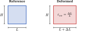
The diagonal components of the strain tensor, called normal strains, describe stretching or compression along the coordinate axes. Consider a small line element of length \(\mathrm{d}x\) oriented along the \(x\)-axis in the reference configuration. After deformation, the \(x\)-component of this element becomes \[\mathrm{d}x' = \mathrm{d}x + u_x(x + \mathrm{d}x, y, z) - u_x(x, y, z) \approx \mathrm{d}x + \frac{\partial u_x}{\partial x}\mathrm{d}x = (1 + \varepsilon_{xx})\mathrm{d}x.\] The normal strain \(\varepsilon_{xx}\) is therefore the relative change in length of a line element originally aligned with the \(x\)-axis, \[\varepsilon_{xx} = \frac{\mathrm{d}x' - \mathrm{d}x}{\mathrm{d}x} = \frac{\Delta L}{L}.\] Positive normal strain indicates elongation (tension), while negative normal strain indicates contraction (compression). The same interpretation applies to \(\varepsilon_{yy}\) and \(\varepsilon_{zz}\) for line elements along the \(y\)- and \(z\)-axes.
Geometric interpretation of shear strains
The off-diagonal components, called shear strains, describe angular distortion—changes in the angles between line elements that were originally perpendicular. Consider two line elements, one along the \(x\)-axis and one along the \(y\)-axis, meeting at a right angle in the reference configuration. After deformation, these elements are no longer perpendicular; the angle between them changes by an amount related to the shear strain.
To see this, consider the displacement of a point at \((x + \mathrm{d}x, y)\) relative to a point at \((x, y)\). The \(y\)-component of this relative displacement is \[\frac{\partial u_y}{\partial x}\mathrm{d}x,\] which represents a rotation of the originally horizontal line element toward the \(y\)-axis. Similarly, a point at \((x, y + \mathrm{d}y)\) experiences a relative \(x\)-displacement of \((\partial u_x/\partial y)\mathrm{d}y\), rotating the originally vertical line element toward the \(x\)-axis.
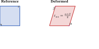
If we denote the rotation of the horizontal edge by angle \(\alpha = \partial u_y/\partial x\) and the rotation of the vertical edge by angle \(\beta = \partial u_x/\partial y\) (both measured in radians and assumed small), then the total change in angle between the two edges is \(\alpha + \beta\). The shear strain component \(\varepsilon_{xy}\) is defined as half of this total angle change, \[\varepsilon_{xy} = \frac{1}{2}(\alpha + \beta) = \frac{1}{2}\left(\frac{\partial u_y}{\partial x} + \frac{\partial u_x}{\partial y}\right).\]
The factor of \(\frac{1}{2}\) in the definition ensures that the strain tensor transforms correctly under coordinate rotations (i.e., as a proper second-rank tensor). In engineering practice, one often encounters the engineering shear strain \(\gamma_{xy} = 2\varepsilon_{xy}\), which equals the total angle change directly. When reading literature or handbooks, it is important to check which definition is being used.
The rotation tensor
The antisymmetric part of the displacement gradient, \[\underline{\omega} = \frac{1}{2}\left(\nabla \vec{u} - (\nabla \vec{u})^T\right),\] describes rigid-body rotation. An antisymmetric tensor satisfies \(\omega_{ij} = -\omega_{ji}\), which means its diagonal elements are zero and it has only three independent components. These can be collected into a vector \(\vec{\omega}\) called the rotation vector, \[\omega_x = \omega_{zy} = \frac{1}{2}\left(\frac{\partial u_z}{\partial y} - \frac{\partial u_y}{\partial z}\right), \quad \text{etc.}\] This rotation vector is related to the curl of the displacement field by \(\vec{\omega} = \frac{1}{2}\nabla \times \vec{u}\).
For small rotations, the rotation tensor \(\underline{\omega}\) represents the local rigid-body rotation of material elements without any change in their shape or size. Pure rotation (without strain) occurs when \(\underline{\varepsilon} = 0\) but \(\underline{\omega} \neq 0\). Conversely, pure deformation (without rotation) occurs when \(\underline{\omega} = 0\) but \(\underline{\varepsilon} \neq 0\).
Physical interpretation as a linear transformation
The strain tensor \(\underline{\varepsilon}\) is a linear transformation that maps a position vector to a displacement vector. For a material point at position \(\vec{r}\) in a uniformly strained body, the displacement is \[\vec{u} = \underline{\varepsilon} \cdot \vec{r}.\] The deformed position is then \[\vec{r}' = \vec{r} + \vec{u} = (\underline{1} + \underline{\varepsilon}) \cdot \vec{r},\] where \(\underline{1}\) is the identity tensor. This shows that the deformation gradient tensor \(\underline{F} = \underline{1} + \underline{\varepsilon}\) transforms reference positions into deformed positions.
Since the strain tensor is symmetric, it can be diagonalized by a rotation of the coordinate system. In the principal coordinate system, the strain tensor takes the form \[\underline{\varepsilon}' = \begin{pmatrix} \varepsilon_1 & 0 & 0 \\ 0 & \varepsilon_2 & 0 \\ 0 & 0 & \varepsilon_3 \end{pmatrix},\] where \(\varepsilon_1\), \(\varepsilon_2\), and \(\varepsilon_3\) are the principal strains. In this coordinate system, there are no shear strains—only normal strains along the principal directions. A cube aligned with the principal axes deforms into a rectangular parallelepiped with edges stretched or compressed by factors \((1 + \varepsilon_1)\), \((1 + \varepsilon_2)\), and \((1 + \varepsilon_3)\).
Volumetric and deviatoric strain
Just as we decomposed the stress tensor into hydrostatic and deviatoric parts, we can decompose the strain tensor similarly. The volumetric strain (or dilatation) is defined as the trace of the strain tensor, \[\varepsilon_\text{vol} = \text{tr}\,\underline{\varepsilon} = \varepsilon_{xx} + \varepsilon_{yy} + \varepsilon_{zz} = \nabla \cdot \vec{u}.\] This quantity represents the relative change in volume of an infinitesimal element. To see this, consider a small cube with edges \(\mathrm{d}x\), \(\mathrm{d}y\), \(\mathrm{d}z\) that deforms into a rectangular parallelepiped with edges \((1+\varepsilon_{xx})\mathrm{d}x\), \((1+\varepsilon_{yy})\mathrm{d}y\), \((1+\varepsilon_{zz})\mathrm{d}z\). The ratio of deformed to reference volume is \[\frac{V'}{V} = (1+\varepsilon_{xx})(1+\varepsilon_{yy})(1+\varepsilon_{zz}) \approx 1 + \varepsilon_{xx} + \varepsilon_{yy} + \varepsilon_{zz} = 1 + \varepsilon_\text{vol},\] where we have neglected products of small strains. Thus \(\varepsilon_\text{vol} = (V' - V)/V = \Delta V/V\).
The deviatoric strain tensor is defined as \[\underline{e} = \underline{\varepsilon} - \frac{1}{3}\varepsilon_\text{vol}\,\underline{1},\] which has zero trace by construction. The deviatoric strain represents shape change at constant volume (distortion), while the volumetric part represents volume change without shape change (dilatation). This decomposition will prove useful when we discuss Hooke’s law, where the volumetric and deviatoric responses are governed by different elastic constants.
Example: Uniform extension
Consider a bar being stretched uniformly along the \(x\)-axis. If the bar has length \(L\) and is stretched to length \(L + \Delta L\), the displacement field is \[u_x = \frac{\Delta L}{L} x, \quad u_y = -\nu \frac{\Delta L}{L} y, \quad u_z = -\nu \frac{\Delta L}{L} z,\] where \(\nu\) is Poisson’s ratio (which we will discuss in Chapter 13). The strain tensor is \[\underline{\varepsilon} = \frac{\Delta L}{L} \begin{pmatrix} 1 & 0 & 0 \\ 0 & -\nu & 0 \\ 0 & 0 & -\nu \end{pmatrix}.\] The axial strain is \(\varepsilon_{xx} = \Delta L/L\), and the transverse strains are \(\varepsilon_{yy} = \varepsilon_{zz} = -\nu \Delta L/L\). The volumetric strain is \[\varepsilon_\text{vol} = (1 - 2\nu)\frac{\Delta L}{L}.\] For most materials \(0 < \nu < 0.5\), so the volumetric strain is positive (the bar expands in volume when stretched). For an incompressible material (\(\nu = 0.5\)), the volumetric strain is zero—the bar gets longer and thinner such that its volume remains constant.
Compatibility condition
The compatibility condition is a constraint that every valid strain field must satisfy. It ensures that the strain field can actually arise from a continuous displacement field.
Why compatibility is needed
In elasticity, we often work with stress and strain fields rather than displacements. When we calculate strains from stresses using Hooke’s law, we need to ensure that these strains are compatible—that is, they can be integrated to give a single-valued, continuous displacement field.
Not every arbitrary strain field can arise from an actual deformation. The strain components must satisfy certain differential relationships to ensure geometric consistency.
Derivation
For plane problems, the strain-displacement relations are: \[\begin{align} \varepsilon_{xx} &= \frac{\partial u_x}{\partial x} \\ \varepsilon_{zz} &= \frac{\partial u_z}{\partial z} \\ \varepsilon_{xz} &= \frac{1}{2}\left(\frac{\partial u_x}{\partial z} + \frac{\partial u_z}{\partial x}\right) \end{align}\]
We can eliminate the displacement components by taking appropriate derivatives. From the first equation: \[\frac{\partial^2 \varepsilon_{xx}}{\partial z^2} = \frac{\partial^3 u_x}{\partial x \partial z^2}\]
From the second equation: \[\frac{\partial^2 \varepsilon_{zz}}{\partial x^2} = \frac{\partial^3 u_z}{\partial z \partial x^2}\]
From the third equation: \[2\frac{\partial^2 \varepsilon_{xz}}{\partial x \partial z} = \frac{\partial^3 u_x}{\partial x \partial z^2} + \frac{\partial^3 u_z}{\partial z \partial x^2}\]
Combining these, we obtain the compatibility condition for plane problems: \[\begin{equation} \frac{\partial^2 \varepsilon_{xx}}{\partial z^2} + \frac{\partial^2 \varepsilon_{zz}}{\partial x^2} = 2\frac{\partial^2 \varepsilon_{xz}}{\partial x \partial z} \end{equation}\]
This is a necessary and sufficient condition (in a simply-connected domain) for a strain field to be derivable from a single-valued displacement field.
Geometric interpretation: The jigsaw puzzle analogy
The compatibility condition has a simple geometric explanation. Imagine a jigsaw puzzle that you deform in its assembled state. Even in the deformed state, all pieces must still fit together—there can be no gaps or overlaps.
If you were to deform each puzzle piece independently (ignoring the constraint that they must fit together), you could assign arbitrary strains to each piece. But when you try to reassemble the puzzle, the pieces might not fit.
The compatibility condition ensures that neighboring material elements deform in a way that they remain geometrically compatible—they continue to fit together after deformation. This is mathematically equivalent to requiring that the displacement field be single-valued and continuous.
The compatibility condition is analogous to a well-known result in vector calculus: the curl of a gradient is zero (\(\nabla \times (\nabla \phi) = 0\)).
Just as this condition ensures that a vector field is the gradient of some scalar potential, the compatibility conditions ensure that a strain tensor field is the symmetrized gradient of some displacement vector field.
Compatibility in 3D
In three dimensions, there are six compatibility equations (one for each pair of strain components). The 2D compatibility equation derived above is a special case that applies when quantities are independent of the \(y\)-direction.
Practical importance
In solving elasticity problems:
Displacement-based methods: If we solve for displacements directly, compatibility is automatically satisfied (since we compute strains as derivatives of displacements)
Stress-based methods: If we work with stress fields (e.g., using the Airy stress function), we must explicitly verify that the resulting strains satisfy compatibility
The compatibility condition plays a central role in the mathematical structure of elasticity theory and is essential for methods like the Airy stress function approach used in fracture mechanics.
This chapter introduced the kinematics of a continuum:
- Displacement field: \(\vec{u}(\vec{r}) = \vec{r}\,' - \vec{r}\)
- Displacement gradient: \(\nabla\vec{u} = \underline{\varepsilon} + \underline{\omega}\) with strain \(\underline{\varepsilon} = \frac{1}{2}(\nabla\vec{u} + (\nabla\vec{u})^T)\) and rotation \(\underline{\omega} = \frac{1}{2}(\nabla\vec{u} - (\nabla\vec{u})^T)\)
- Normal strains \(\varepsilon_{ii}\) measure relative elongation, shear strains \(\varepsilon_{ij}\) (\(i\neq j\)) half the change of a right angle
- Volumetric strain: \(\mathrm{tr}\,\underline{\varepsilon}\) is the relative change of volume
- Compatibility: in 2D \(\varepsilon_{xx,zz} + \varepsilon_{zz,xx} = 2\varepsilon_{xz,xz}\) ensures that a strain field derives from a continuous displacement field