After completing this chapter, you should be able to:
Distinguish isostatic and hyperstatic (statically indeterminate) beams
Solve hyperstatic beams by integrating \(EI w'''' = q\) with the support reaction as a Dirac load
Compute the elastic energy of a beam and apply Castigliano’s theorem
Derive the principle of virtual forces \(\delta = \int M m/(EI)\,\mathrm{d}x\)
Apply the force (flexibility) method and the Müller-Breslau formula
From isostatic to hyperstatic
In the previous chapters we dealt with isostatic (statically determinate) beams: the equilibrium conditions were sufficient to compute all reactions and internal forces. Many structures — and many microstructures — are hyperstatic (statically indeterminate): they have more constraints than strictly necessary, \(D = 3n - \sum c_i < 0\). The degree of indeterminacy \(-D\) counts the reactions that equilibrium cannot determine. To find them we must look at the deformation of the structure: every redundant support imposes a kinematic condition (e.g. \(w = 0\) at a roller) that provides the missing equation.
This chapter presents two routes:
integrating the Euler–Bernoulli equation \(EI\,w'''' = q\) with the redundant reactions as unknown point loads;
energy methods — Castigliano’s theorem and the principle of virtual forces — which lead to the force method (flexibility method) and the Müller-Breslau formula.
The first route is direct for a single beam. The second is more convenient for structures made of several beams and internal constraints.
Hyperstatic beams with the Euler–Bernoulli equation
Consider a cantilever of length \(\ell\), clamped at \(x=0\), with an additional roller at \(x = \ell/2\) and a downward force \(F\) at the free end \(x=\ell\). The structure has \(D = 3 - (3+1) = -1\): it is hyperstatic of degree one.
We treat the unknown roller reaction \(R\) (upward) as a point load, \(q(x) = -R\,\delta(x - \ell/2)\), and integrate \[EI\,w'''' = -R\,\delta\!\left(x - \tfrac{\ell}{2}\right).\] Four integrations give, with \(\langle x - \ell/2\rangle^n \equiv (x-\ell/2)^n\,\theta(x-\ell/2)\), \[\begin{aligned}
EI\,w''' &= -R\,\theta\!\left(x-\tfrac{\ell}{2}\right) + C_1, \\
EI\,w'' &= -R\,\langle x-\tfrac{\ell}{2}\rangle + C_1 x + C_2, \\
EI\,w' &= -\tfrac{R}{2}\langle x-\tfrac{\ell}{2}\rangle^2 + \tfrac{C_1}{2}x^2 + C_2 x + C_3, \\
EI\,w &= -\tfrac{R}{6}\langle x-\tfrac{\ell}{2}\rangle^3 + \tfrac{C_1}{6}x^3 + \tfrac{C_2}{2}x^2 + C_3 x + C_4.
\end{aligned}\] We have five unknowns (\(C_1,\dots,C_4\) and \(R\)) and five conditions:
The clamp gives \(C_3 = C_4 = 0\). The free end gives \(R - C_1 = F\) and \(-R\ell/2 + C_1\ell + C_2 = 0\), i.e. \(C_1 = R - F\) and \(C_2 = F\ell - R\ell/2\). Finally, the roller condition \(w(\ell/2) = 0\) reads \(C_1\ell/6 + C_2 = 0\), so \[\frac{(R-F)\,\ell}{6} + F\ell - \frac{R\ell}{2} = 0 \quad\Rightarrow\quad R = \frac{5}{2}F.\] The roller carries more than twice the applied load; the clamp pulls down with \(Q(0) = -C_1 = F - R = -\tfrac{3}{2}F\) and carries the moment \(M(0) = -C_2 = F\ell/4\). The tip deflection is \[w(\ell) = \frac{7F\ell^3}{96\,EI},\] about a fifth of the \(F\ell^3/(3EI)\) of the cantilever without the roller.
The extra kinematic condition provided exactly the extra equation. This works well for one beam, but the bookkeeping grows quickly with the number of beams and internal hinges. The energy methods below are often more convenient.
Elastic energy of a beam
A linear spring with stiffness \(k\), stretched by \(x\) under the force \(F = kx\), stores the elastic energy \[U = \int_0^x k\,x'\,\mathrm{d}x' = \frac{1}{2}k x^2 = \frac{1}{2}F x,\] i.e. half of the product of force and displacement (the area under the linear force–displacement curve).
A beam element of length \(\mathrm{d}x\) behaves like a rotational spring: the moment \(M\) rotates its two faces relative to each other by \(\chi\,\mathrm{d}x\). With \(M = EI\chi\) the stored energy is \(\frac{1}{2}M\chi\,\mathrm{d}x = \frac{M^2}{2EI}\mathrm{d}x\). The elastic (strain) energy of a beam in bending is therefore \[\boxed{U = \int_0^\ell \frac{M(x)^2}{2EI}\,\mathrm{d}x.}\] In general all three conjugate pairs contribute, \(U = \int \left(\frac{N^2}{2EA} + \frac{Q^2}{2GA^*} + \frac{M^2}{2EI}\right)\mathrm{d}x\). For slender beams in bending the last term dominates by far, and we keep only that one.
Castigliano’s theorem
Alberto Castigliano (1847–1884) showed that for a linear elastic structure, the derivative of the elastic energy with respect to an applied force \(F_i\) is the displacement \(\delta_i\) of the point of application of that force, in the direction of the force: \[\boxed{\delta_i = \frac{\partial U}{\partial F_i}.}\] For the spring, \(U = F^2/(2k)\) and \(\partial U/\partial F = F/k = x\). For a beam, we differentiate under the integral, \[\delta_i = \int_0^\ell \frac{M}{EI}\,\frac{\partial M}{\partial F_i}\,\mathrm{d}x.\]
Example. A cantilever of length \(\ell\) (clamped at \(x=0\)) carries a force \(F\) at the free end. The bending moment is \(M(x) = -F(\ell - x)\), so \[U = \int_0^\ell \frac{F^2(\ell-x)^2}{2EI}\,\mathrm{d}x = \frac{F^2\ell^3}{6EI}, \qquad w(\ell) = \frac{\partial U}{\partial F} = \frac{F\ell^3}{3EI},\] the same result that we obtained by integrating the Euler–Bernoulli equation in Chapter 7.
Principle of virtual forces
Castigliano’s theorem gives the displacement only where a force acts. To compute the displacement \(\delta\) at any point, we apply a fictitious force \(\bar{F}\) there, in the direction of the displacement we look for. By linearity, the bending moment of the structure is the sum of the moment \(M(x)\) due to the real loads and \(\bar{F}\) times the moment \(m(x)\) due to a unit force at the point: \[M_\text{tot}(x) = M(x) + \bar{F}\,m(x).\] Castigliano’s theorem gives \[\delta = \frac{\partial}{\partial\bar{F}}\int_0^\ell \frac{(M + \bar{F}m)^2}{2EI}\,\mathrm{d}x = \int_0^\ell \frac{(M + \bar{F}m)\,m}{EI}\,\mathrm{d}x,\] and setting the fictitious force back to zero, \[\boxed{\delta = \int_0^\ell \frac{M(x)\,m(x)}{EI}\,\mathrm{d}x.}\] To find a rotation instead of a displacement, we use a unit couple instead of a unit force.
This is the principle of virtual forces (or unit-load method). It is the dual of the principle of virtual work of Chapter 6. There we combined real forces with virtual displacements. Here we combine a virtual (unit) force system \(m\), which only needs to satisfy equilibrium, with the real curvature \(\chi = M/EI\): \[1\cdot\delta = \int_0^\ell m\,\chi\,\mathrm{d}x.\]
Example. The midspan deflection of a simply supported beam of length \(\ell\) under a uniform load \(q_0\): the real moment is \(M(x) = \frac{q_0}{2}x(\ell - x)\). A unit downward force at midspan produces \(m(x) = x/2\) for \(x \le \ell/2\) (and symmetrically on the other half). Hence \[w\!\left(\tfrac{\ell}{2}\right) = 2\int_0^{\ell/2} \frac{1}{EI}\,\frac{q_0}{2}x(\ell-x)\,\frac{x}{2}\,\mathrm{d}x = \frac{q_0}{2EI}\left[\frac{\ell x^3}{3} - \frac{x^4}{4}\right]_0^{\ell/2} = \frac{5\,q_0\ell^4}{384\,EI}.\]
The force method
The force method (flexibility method, method of consistent deformations) treats the redundant reactions as unknown loads on a statically determinate structure.
Degree of indeterminacy: \(n = -D\).
Primary structure (“0”): remove \(n\) redundant constraints so that the structure becomes isostatic (and is still not a mechanism). Compute its bending moment \(M_0(x)\) under the real loads.
Redundants (“X”): the forces \(X_1,\dots,X_n\) of the removed constraints. For each, compute the moment \(m_i(x)\) of the primary structure loaded only by a unit force in place of \(X_i\).
Superposition: the real structure is the primary structure plus the redundants, \[M(x) = M_0(x) + \sum_i X_i\,m_i(x).\]
Compatibility: the removed constraints must be respected, e.g. zero displacement at a removed roller. With the principle of virtual forces, the displacement at constraint \(i\) is \(\int M\,m_i/(EI)\,\mathrm{d}x = 0\), i.e. \[\delta_{i0} + \sum_j X_j\,\delta_{ij} = 0, \qquad \delta_{i0} = \int_0^\ell \frac{M_0\,m_i}{EI}\,\mathrm{d}x, \quad \delta_{ij} = \int_0^\ell \frac{m_i\,m_j}{EI}\,\mathrm{d}x.\]
For one redundant, the compatibility condition \(\delta_{10} + X\,\delta_{11} = 0\) gives the Müller-Breslau formula\[\boxed{X = -\frac{\displaystyle\int_0^\ell \frac{M_0\,m}{EI}\,\mathrm{d}x}{\displaystyle\int_0^\ell \frac{m^2}{EI}\,\mathrm{d}x}.}\] A positive \(X\) means that the redundant acts in the direction we assumed for the unit force.
Example: two-span continuous beam
Consider a continuous beam of total length \(\ell\) with constant \(EI\):
Supports: hinge at \(A\) (\(x=0\)), roller at \(B\) (\(x=\ell/2\)), roller at \(C\) (\(x=\ell\));
Load: uniform line load \(q_0\), downward, over the whole length.
With one body and \(2+1+1 = 4\) constraints, \(D = 3 - 4 = -1\): the beam is hyperstatic of degree one.
Primary structure. We remove the middle roller \(B\); what remains is a simply supported beam of length \(\ell\). Integrating \(Q' = -q_0\), \(M' = Q\) with \(M(0) = M(\ell) = 0\) (Chapter 4) gives \[M_0(x) = \frac{q_0}{2}\,x\,(\ell - x).\]
Unit load. We apply an upward unit force at \(B\) in place of the redundant \(X = R_B\). The supports react with \(1/2\) downward each, and \[m(x) = \begin{cases} -\dfrac{x}{2} & 0 \le x \le \ell/2 \\[1ex] -\dfrac{\ell - x}{2} & \ell/2 \le x \le \ell.\end{cases}\]
Müller-Breslau. By symmetry we integrate over the left half and double: \[\int_0^\ell M_0\,m\,\mathrm{d}x = -2\int_0^{\ell/2}\frac{q_0}{2}x(\ell-x)\frac{x}{2}\,\mathrm{d}x = -\frac{5\,q_0\ell^4}{384}, \qquad \int_0^\ell m^2\,\mathrm{d}x = 2\int_0^{\ell/2}\frac{x^2}{4}\,\mathrm{d}x = \frac{\ell^3}{48}.\] Therefore \[X = R_B = -\frac{-5q_0\ell^4/384}{\ell^3/48} = \frac{5}{8}\,q_0\ell.\]\(X\) is positive, so the middle support indeed pushes upward. The two integrals are nothing but the midspan deflection of the primary structure under \(q_0\), \(5q_0\ell^4/(384EI)\), and under a unit force, \(\ell^3/(48EI)\): the redundant is chosen such that the two cancel.
Reactions. By symmetry \(R_A = R_C\), and vertical equilibrium \(R_A + R_B + R_C = q_0\ell\) gives
Support
Reaction (upward)
\(A\) (left)
\(\frac{3}{16}q_0\ell\)
\(B\) (middle)
\(\frac{5}{8}q_0\ell\)
\(C\) (right)
\(\frac{3}{16}q_0\ell\)
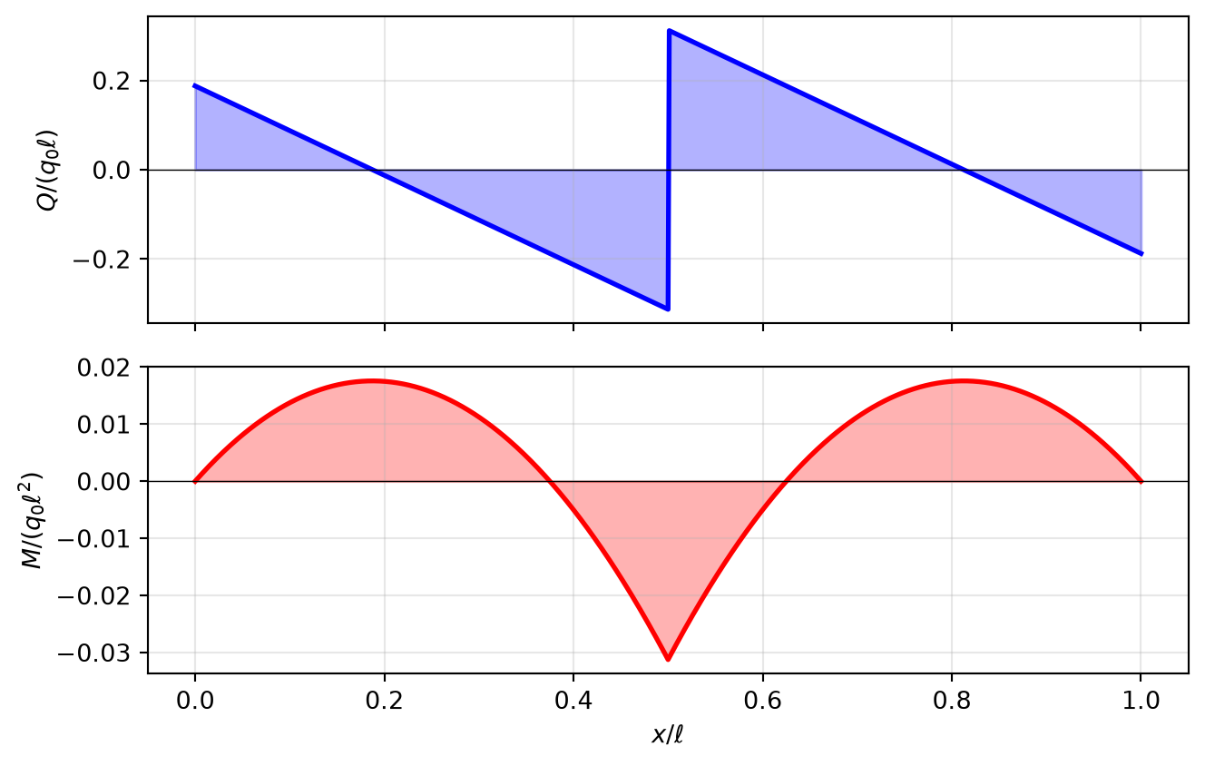
Internal forces. Superposition \(M = M_0 + X m\), or equivalently integration with the reactions, gives
for \(0 \le x < \ell/2\): \(Q(x) = \frac{3}{16}q_0\ell - q_0 x\), \(\quad M(x) = \frac{3}{16}q_0\ell x - \frac{q_0x^2}{2}\);
for \(\ell/2 < x \le \ell\): \(Q(x) = \frac{3}{16}q_0\ell - q_0 x + \frac{5}{8}q_0\ell\), \(\quad M(x) = \frac{3}{16}q_0\ell x - \frac{q_0 x^2}{2} + \frac{5}{8}q_0\ell\left(x - \frac{\ell}{2}\right)\).
The shear force jumps by \(R_B\) at the middle support, where the bending moment reaches its extreme value \(M(\ell/2) = -q_0\ell^2/32\) (top in tension), see Figure 1.
Code
import numpy as npimport matplotlib.pyplot as pltx = np.linspace(0, 1, 801) # x / lRA, RB =3/16, 5/8# in units of q0 lright = (x >0.5).astype(float)Q = RA - x + RB * right # Q / (q0 l)M = RA * x - x**2/2+ RB * (x -0.5) * right # M / (q0 l^2)fig, (ax1, ax2) = plt.subplots(2, 1, figsize=(7, 4.5), sharex=True)ax1.fill_between(x, 0, Q, alpha=0.3, color='blue')ax1.plot(x, Q, 'b-', lw=2)ax1.axhline(0, color='k', lw=0.5)ax1.set_ylabel(r'$Q / (q_0 \ell)$')ax1.grid(True, alpha=0.3)ax2.fill_between(x, 0, M, alpha=0.3, color='red')ax2.plot(x, M, 'r-', lw=2)ax2.axhline(0, color='k', lw=0.5)ax2.set_xlabel(r'$x / \ell$')ax2.set_ylabel(r'$M / (q_0 \ell^2)$')ax2.grid(True, alpha=0.3)plt.tight_layout()plt.show()
Figure 1: Shear force and bending moment of the two-span continuous beam under uniform load \(q_0\) (total length \(\ell\)).
NoteChapter Summary
This chapter introduced methods for statically indeterminate beams:
Hyperstatic beams (\(D<0\)) have more reactions than equilibrium equations; each redundant constraint adds a kinematic condition
Euler–Bernoulli route: treat redundant reactions as Dirac loads in \(EIw'''' = q\) and use all kinematic and static boundary conditions