3. Constraints and virtual work

Learning Objectives

After completing this chapter, you should be able to:

State the principle of virtual work and derive the rigid-body equilibrium conditions from it
Identify different types of supports (rollers, hinges, fixed) and their constraint degrees
Calculate the degree of static determinacy $D = 3n - \sum c_i$ for 2D structures
Determine the instantaneous center of rotation to verify if constraints are properly placed

In Chapter 1 we wrote down the equilibrium of a rigid body by balancing forces and moments. In Chapter 2 we described how a rigid body can move. In this chapter we combine the two: the principle of virtual work derives the equilibrium conditions a second time, starting from the kinematics. We will use exactly the same strategy again for beams (Chapter 6) and for the continuum (Chapter 12). We then use the kinematic viewpoint to classify supports and to decide whether a structure can move.

Virtual work

Virtual displacements

From Chapter 2, the velocity of any point $P$ of a rigid body is \[\vec{v}_P = \vec{v}_O + \vec{\omega}\times\vec{r}_{OP},\] where $O$ is a reference point of the body. Multiplying by a small time increment $\mathrm{d}t$ gives the small displacement of $P$. We now imagine such a small displacement, without asking whether it actually happens: \[\delta\vec{u}_P = \delta\vec{u}_O + \delta\vec{\theta}\times\vec{r}_{OP}. \tag{1}\] A virtual displacement $\delta\vec{u}$ is an infinitesimal, imagined displacement of the body that is compatible with its kinematics (here: rigid) and with its constraints. The forces are held fixed while we imagine it. For a rigid body, a virtual displacement is fully described by a virtual translation $\delta\vec{u}_O$ and a virtual rotation $\delta\vec{\theta}$ — in 2D these are three numbers, $\delta u_{O,x}$, $\delta u_{O,y}$ and $\delta\theta$.

Work and virtual work

The work done by a constant force $\vec{F}$ along a displacement $\vec{u}$ is $W = \vec{F}\cdot\vec{u}$. The virtual work is the work done by the (real) forces along a virtual displacement, \[\delta W = \vec{F}\cdot\delta\vec{u}.\]

The principle of virtual work

Principle of virtual work

A body is in equilibrium if and only if the virtual work of all forces acting on it vanishes for every admissible virtual displacement: \[\delta W = 0 \quad \text{for all admissible } \delta\vec{u}.\]

We split the virtual work into the contributions of external loads, of constraint (reaction) forces and of internal forces, \[\delta W = \delta W_e + \delta W_c + \delta W_i = 0.\] Two simplifications apply:

Perfect constraints (no friction): a reaction force is always perpendicular to the motion that the constraint allows. If the virtual displacement respects the constraints, $\delta W_c = 0$.
Rigid body: internal forces come in action–reaction pairs acting along the line that connects two material points. In a rigid body the distance between the points does not change, so the pair does no work, $\delta W_i = 0$.

For a rigid body with perfect constraints, the principle therefore reduces to \[\delta W_e = 0.\]

Equilibrium of a rigid body from virtual work

Let the external loads be distributed over the body, with an infinitesimal force $\mathrm{d}\vec{f}_e$ acting on the material at point $P$. Inserting the rigid-body virtual displacement Equation 1 gives \[\delta W_e = \int_V \mathrm{d}\vec{f}_e\cdot\left(\delta\vec{u}_O + \delta\vec{\theta}\times\vec{r}_{OP}\right) = \delta\vec{u}_O\cdot\int_V \mathrm{d}\vec{f}_e + \delta\vec{\theta}\cdot\int_V \vec{r}_{OP}\times\mathrm{d}\vec{f}_e,\] where we used the cyclic property of the scalar triple product, $\vec{a}\cdot(\vec{b}\times\vec{c}) = \vec{b}\cdot(\vec{c}\times\vec{a})$. The two integrals are the resultant force and the resultant moment about $O$, \[\vec{F} = \int_V \mathrm{d}\vec{f}_e, \qquad \vec{M}_O = \int_V \vec{r}_{OP}\times\mathrm{d}\vec{f}_e,\] so that \[\delta W_e = \vec{F}\cdot\delta\vec{u}_O + \vec{M}_O\cdot\delta\vec{\theta}.\] The virtual translation and the virtual rotation can be chosen independently and arbitrarily. $\delta W_e = 0$ for all of them is only possible if \[\boxed{\vec{F} = 0 \quad\text{and}\quad \vec{M}_O = 0.}\] These are exactly the equilibrium conditions of Chapter 1. In 2D we obtain three scalar equations ($F_x = 0$, $F_y = 0$, $M = 0$), one for each rigid-body degree of freedom. The force $\vec{F}$ does work on the translation, the moment $\vec{M}$ does work on the rotation: $\vec{F}$ and $\delta\vec{u}_O$, $\vec{M}$ and $\delta\vec{\theta}$ are conjugate pairs.

Example: reaction of a simply supported beam

The principle of virtual work is useful in practice because we can pick a virtual displacement that involves only the unknown we are interested in. Consider a beam of length $L$ with a hinge at $A$ ($x=0$), a roller at $B$ ($x=L$) and a downward force $F$ at $x=a$. To find the reaction $R_B$ (upward), we remove the roller and replace it by the force $R_B$. The beam can now rotate about $A$; we give it a small virtual rotation $\delta\theta$ such that the point at $x$ moves downward by $x\,\delta\theta$. The hinge reaction does no work (point $A$ does not move), so \[\delta W_e = F\,a\,\delta\theta - R_B\,L\,\delta\theta = 0 \quad\Rightarrow\quad R_B = \frac{a}{L}F.\] One virtual displacement gives one equation for one unknown. Releasing a constraint and moving the resulting mechanism is a systematic way to compute reactions — and, as we will see in Chapter 6, also internal forces.

The principle also shows the link between kinematics and statics that we use in the rest of this chapter: every constraint removes one virtual displacement and introduces one reaction force that does work on it.

Constraints and degrees of freedom

The condition of static equilibrium that we discussed in Chapter 1 does not mean that the body is immovable. As you saw in the previous section, the body still can translate and rotate; in a two-dimensional case an object can have three kinematics degrees of freedom (DoFs): two orthogonal translational displacements along x- and y- axes, and one rotation around z-axis. The motion of the body can be constrained by eliminating some DoFs with the help of supports (Figure 1). Depending on the type of support, one, two, or all three DoFs can be removed. The kinematic constraints imposed by supports trigger so-called reaction forces, or simply reactions. Note that if exactly all degrees of freedom are removed, the system is called statically determinate or isostatic.

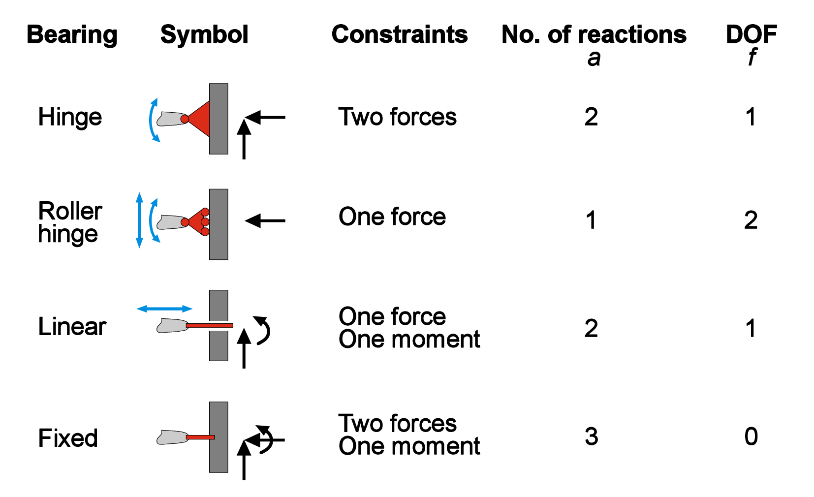
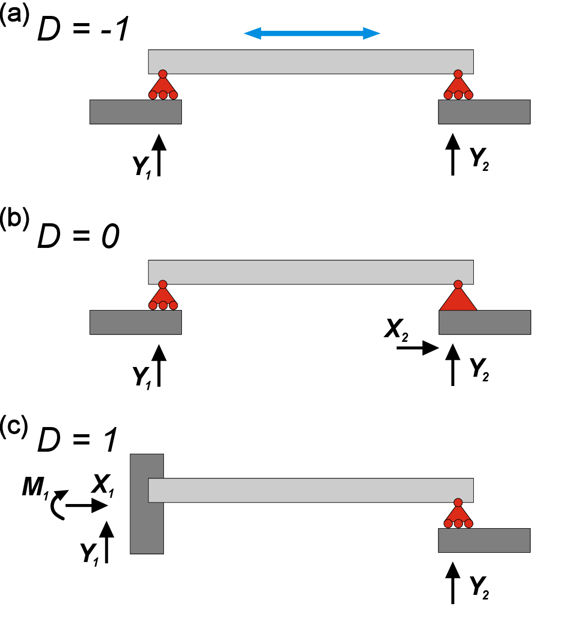
Figure 1: The most common types of supports and corresponding number of constraints $c$ and degrees of freedom $f$.

As you can see, the sum of the degrees of constraints $c_i$ and DoFs $f_i$ is always equal to 3 (for 2D case). This is a necessary (but not a sufficient!) condition for a statically determinate system with one body and $m$ constraints. Namely, \[3-\sum _{i}^{m}{c_i}=0 \]For more general 2D system with $n$ connected bodies \[3n-\sum _{i}^{m}{c_i}=0. \] By having $n$ bodies, $m$ constraints of degree $c_i$, we can distinguish three different cases for 2D force systems defined by the value of $D$, where \[D=3n-\sum _{i}^{m}{c_i} \label {eq:D} \]We know that a determinate (or isostatic) system must have $D=0$ (Figure 2 b). If $D>0$, then the system is movable or kinematically indeterminate since it has unrestricted DoF (Figure 2 a). If $D<0$, then the system is called statically indeterminate or hyperstatic - the system is immovable and contains extra reactions that can be removed (Figure 2 c).

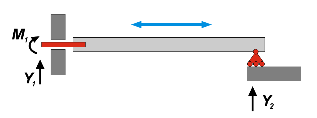
Figure 2: Movable (a), isostatic (b) and hyperstatic (c) structure.

Again, we need to emphasize that above-mentioned mathematical precondition is a necessary, but not sufficient, requirement. One exception from this rule is the system with two and one reactions in the left and right supports respectively shown in Figure 3. Here, we have $D=0$, which usually corresponds to determinate system. However, it is clear that the beam can move freely in a horizontal direction, therefore it has 1 DoF! In this specific case, force vectors $Y_1$ and $Y_2$ are parallel, and they both can compensate only vertical direction of action, while the horizontal movement is not restricted. It means that the constraints are ill placed. A systematic way to determine if constraints are well placed consists in determining the Instantaneous Center of Rotation.

Figure 3: Example of movable force system with $D=0$. Parallel vertical forces $Y_1$ and $Y_2$ cannot restrict horizontal movement of the beam.

Instantaneous Center of Rotation.

In planar (2D) kinematics, the Instantaneous Center of Rotation $C$ is a point in or outside a rigid body about which the entire body appears to rotate at a given instant of time.

At that instant, all points of the body have velocities that are equivalent to those of a pure rotation about the $C$.

Consider a rigid body moving in a plane. At any instant, the motion can be described as a combination of translation and rotation. The instantaneous center of rotation is defined as the point of the body (or its extension) that has zero velocity at that instant. \[v_{C} = 0\] All other points of the body move as if rotating about this point.

Let the body have an angular velocity $$ (positive counterclockwise). If $P$ is a point on the body and $r_{P/C}$ is the position vector from the $C$ to $P$, the velocity of $P$ is given by \[\vec{v}_P = \vec{\omega } \times \vec{r}_{P/C}\] In planar motion, this reduces to the scalar relation: \[v_P = \omega \, r_{P/C}\] where $r_{P/C}$ is the distance between $P$ and the instantaneous center.

If the instantaneous center of rotation is located at infinity, the motion is a pure translation without rotation (if $r_{P/C} \to \infty$ then $ $).

Thus, given an assembly of rigid bodies, it is appropriate to verify the existence of $C$ in order to determine if a structure is really static ($D\le 0$) or if some constraints are ill placed, as in the example of Figure 3.

The existence of $C$ can be determined by looking at the constraints. Single constraints allow for infinite possible centers of rotations: all the points of the line perpendicular to the direction of motion of the roller, and all the points at the infinity for the rotation lock. Double constraints allow only one center of rotations: the center of the hinge or the point at the infinity in the direction perpendicular to the movement of the linear bearing. Triple constraints do not allow any possible center of rotation.

For a single constrained rigid body, if there is a point in common among all possible instantaneous centers of rotations of each constraint, that point is $C$ and

the body is kinematically indeterminate. For example, in the structure depicted in Figure 3, the linear bearing admits only one possible $C$ at the infinity, in the direction perpendicular to axis of the beam, and the roller allows infinite ICRs normal to the roller, including of course the point at the infinity. Thus, both constraints admit $C$ at the infinity perpendicular to the beam, which is indeed the point around which the beam can freely rotate (i.e. the beam can translate rigidly horizontally).

When moving from a single beam to systems of rigid bodies, it becomes necessary to distinguish between different definitions of the instantaneous center of rotation:

The absolute center of rotation, denoted as $C_i$, is the point around which the $i$-th body rotates. This point is therefore fixed with respect to a global reference system, and its existence is only possible in mechanisms that are kinematically undetermined and statically impossible ($D>0$).
The relative center of rotation between two bodies is the point $C_{ij}$ such that, when observing body $i$ from a reference frame attached to body $j$, the latter would appear to be at rest while the former rotates about $C_{ij}$. External constraints affect the position of the absolute center, while internal constraints affect that of the relative center, in a way entirely analogous to what has already been discussed.

For an assembly consisting of two rigid bodies, we can use the first theorem of kinematic chains: given a structure consisting of two rigid bodies $i$ and $j$, a necessary and sufficient condition for it to be a mechanism is that the instantaneous centers of rotation $C_i$, $C_j$, and $C_{ij}$ are aligned.

Chapter Summary

This chapter connected the statics and the kinematics of rigid bodies:

Virtual displacement: an imagined infinitesimal displacement compatible with the kinematics and the constraints; for a rigid body $\delta\vec{u}_P = \delta\vec{u}_O + \delta\vec{\theta}\times\vec{r}_{OP}$
Principle of virtual work: equilibrium $\Leftrightarrow$ $\delta W = 0$ for every admissible virtual displacement; with perfect constraints and a rigid body, $\delta W_e = \vec{F}\cdot\delta\vec{u}_O + \vec{M}_O\cdot\delta\vec{\theta} = 0$, hence $\vec{F} = 0$, $\vec{M}_O = 0$
Supports: remove degrees of freedom; rollers (1 constraint), hinges (2), fixed supports (3)
Static determinacy: $D = 3n - \sum c_i$; $D=0$ isostatic, $D>0$ movable, $D<0$ hyperstatic
Instantaneous center of rotation: a point about which a body instantaneously rotates; it tells whether constraints are properly placed

Equilibrium of forces (Chapter 1), kinematics (Chapter 2) and virtual work (this chapter) are the three steps that we will repeat for beams and for the continuum.