2. Rigid-body kinematics
After completing this chapter, you should be able to:
- Describe a rigid-body motion as a combination of translation and rotation
- Transform vector components between rotated coordinate systems using the rotation matrix \(\underline{R}\)
- Derive the rigid-body velocity field \(\vec{v}_P = \vec{v}_O + \vec{\omega}\times\vec{r}_{P/O}\)
Rigid-body kinematics
Every rigid body motion in 3D space is a composition of translations and rotations. While translations are trivial, we need to discuss rotations in detail.
Coordinate transformation of a vector
A rotation \(\mathcal{R}\) is a linear operation that does not affect the length (or norm) of the vector, \(|\mathcal{R}\vec{r}|=|\vec{r}|\). We distinguish between the operation \(\mathcal{R}\) and its representation in the form of a matrix \(\underline{R}\) (we use underlines to denote matrices and second-order tensors throughout these notes). We can write the rotation as the product of this matrix with a vector, \[|\underline{R}\cdot \vec{r}| = ( R_{ij} r_j R_{ik} r_k )^{1/2} = ( r_j R^T_{ji} R_{ik} r_k )^{1/2} = \left ( \vec{r}\cdot \underline{R}^T\cdot \underline{R}\cdot \vec{r} \right )^{1/2}. \] This must be equal equal to \(|\vec{r}|\), which implies \(\underline{R}^T\cdot \underline{R}=\underline{I}\), i.e. if the rotation matrix \(\underline{R}\) is an orthogonal matrix. Here the superscript \(^T\) indicates the transpose operation, \(R^T_{ij}=R_{ji}\), and \(\underline{I}\) is the unit matrix. Note that this relationship implies \(\underline{R}^{-1}=\underline{R}^T\), i.e. the inverse of an orthogonal matrix is simply its transpose.
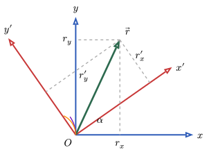
Figure 1 illustrates the rotation of a coordinate system. The same vector \(\vec{r}\) can be expressed in terms of components in the original coordinate system \((\hat{x}, \hat{y})\) or in the rotated system \((\hat{x}', \hat{y}')\). The rotation matrix \(\underline{R}\) transforms the components from one system to the other while preserving the vector’s length.
Let us assume we want to rotate from a coordinate system with basis vectors \(\hat {x}\), \(\hat {y}\), and \(\hat {z}\) to a primed coordinate system \(\hat {x}'\), \(\hat {y}'\), and \(\hat {z}'\). The rotation operator \(\mathcal{R}\) should transform the basis vectors of the unprimed into the primed system, \[\mathcal{R}\hat {x} = \hat {x}', \quad \mathcal{R}\hat {y} = \hat {y}', \quad \mathcal{R}\hat {z} = \hat {z}'. \] We can construct the rotation matrix from this definition of the action of the rotation on the basis vectors. From the component definition we obtain \[\underline{R} = \begin {pmatrix} R_{xx} & R_{xy} & R_{xz} \\ R_{yx} & R_{yy} & R_{yz} \\ R_{zx} & R_{zy} & R_{zz} \end {pmatrix} = \begin {pmatrix} \hat {x}\cdot \mathcal{R}\hat {x} & \hat {x}\cdot \mathcal{R}\hat {y} & \hat {x}\cdot \mathcal{R}\hat {z} \\ \hat {y}\cdot \mathcal{R}\hat {x} & \hat {y}\cdot \mathcal{R}\hat {y} & \hat {y}\cdot \mathcal{R}\hat {z} \\ \hat {z}\cdot \mathcal{R}\hat {x} & \hat {z}\cdot \mathcal{R}\hat {y} & \hat {z}\cdot \mathcal{R}\hat {z} \end {pmatrix} = \begin {pmatrix} \hat {x}\cdot \hat {x}' & \hat {x}\cdot \hat {y}' & \hat {x}\cdot \hat {z}' \\ \hat {y}\cdot \hat {x}' & \hat {y}\cdot \hat {y}' & \hat {y}\cdot \hat {z}' \\ \hat {z}\cdot \hat {x}' & \hat {z}\cdot \hat {y}' & \hat {z}\cdot \hat {z}' \end {pmatrix}. \] If all vectors are expressed in the coordinate system \(\{\hat {x}, \hat {y}, \hat {z}\}\), then the rotation matrix can be written as \[\underline{R} = (\hat {x}', \hat {y}', \hat {z}'), \] i.e. by stacking the rotated basis vectors as columns. The matrix \(\underline{R}\) is orthogonal, since \[\underline{R}^T\cdot \underline{R} = \begin {pmatrix} \hat {x}'\cdot \hat {x}' & \hat {x}'\cdot \hat {y}' & \hat {x}'\cdot \hat {z}' \\ \hat {y}'\cdot \hat {x}' & \hat {y}'\cdot \hat {y}' & \hat {y}'\cdot \hat {z}' \\ \hat {z}'\cdot \hat {x}' & \hat {z}'\cdot \hat {y}' & \hat {z}'\cdot \hat {z}' \end {pmatrix} = \underline{I}, \] if \(\{\hat {x}', \hat {y}', \hat {z}'\}\) form an orthonormal triad.
For example, a counterclockwise rotation by an angle \(\theta\) about the \(z\)-axis leaves \(\hat {z}\) unchanged: \[\hat {x}' = \begin {pmatrix} \cos \theta \\ \sin \theta \\ 0 \end {pmatrix}, \quad \hat {y}' = \begin {pmatrix} -\sin \theta \\ \cos \theta \\ 0 \end {pmatrix}, \quad \hat {z}' = \begin {pmatrix} 0 \\ 0 \\ 1 \end {pmatrix}. \] The corresponding rotation matrix is \[\label {eq:rotmat3D} \underline{R}_z(\theta ) = \begin {pmatrix} \cos \theta & -\sin \theta & 0 \\ \sin \theta & \cos \theta & 0 \\ 0 & 0 & 1 \end {pmatrix}. \] It is straightforward to verify that \(\underline{R}_z^T \underline{R}_z = \underline{1}\) and \(\det (\underline{R}_z) = 1\).
Similarly, rotations about the \(x\)- and \(y\)-axes are given by \[\begin{align} \underline{R}_x(\theta ) &= \begin {pmatrix} 1 & 0 & 0 \\ 0 & \cos \theta & -\sin \theta \\ 0 & \sin \theta & \cos \theta \end {pmatrix}, \\[6pt] \underline{R}_y(\theta ) &= \begin {pmatrix} \cos \theta & 0 & \sin \theta \\ 0 & 1 & 0 \\ -\sin \theta & 0 & \cos \theta \end {pmatrix}. \end{align}\]
As an example, for a rotation about the \(z\)-axis by an angle \(\theta\), \[\vec{p'} = \underline{R}_z^T(\theta ) \vec{p} = \begin {pmatrix} \cos \theta & \sin \theta & 0 \\ -\sin \theta & \cos \theta & 0 \\ 0 & 0 & 1 \end {pmatrix} \begin {pmatrix} p_x \\ p_y \\ p_z \end {pmatrix}. \]Thus the components in the rotated coordinate system are \[\begin{align} p_x' &= p_x \cos \theta + p_y \sin \theta , \\ p_y' &= -p_x \sin \theta + p_y \cos \theta , \\ p_z' &= p_z. \end{align}\]
Differentiation of the rotation matrix
A rotation matrix \(\underline{R}(t)\) in three-dimensional space describes the orientation of a rotating coordinate frame as a function of time. By definition, a rotation matrix is orthogonal and has unit determinant: \[\underline{R}(t)\underline{R}(t)^T = \underline{I}, \quad \det \underline{R}(t) = 1. \] Differentiating the orthogonality condition with respect to time yields \[\dot {\underline{R}}(t)\underline{R}(t)^T + \underline{R}(t)\dot {\underline{R}}(t)^T = \underline{0}. \tag{1}\] This equation expresses the fact that the product \(\dot {\underline{R}}(t)\underline{R}(t)^T\) is skew-symmetric. Indeed, multiplying Equation 1 from the right by \(\underline{R}(t)\) gives \[\dot {\underline{R}}(t) = \underline{\Omega }(t)\underline{R}(t), \] where we define \[\underline{\Omega }(t) = \dot {\underline{R}}(t)\underline{R}(t)^T. \] Taking the transpose, \[\underline{\Omega }(t)^T = \underline{R}(t)\dot {\underline{R}}(t)^T, \] so that \(\underline{\Omega }(t)\) is a skew-symmetric matrix, since
\[\underline{\Omega }(t) + \underline{\Omega }(t)^T = \underline{0}. \] Now, a \(3\times 3\) skew-symmetric matrix has only three independent components, which can be associated with the components of the angular velocity vector \(\vec{\omega}(t)\). We therefore write \[\underline{\Omega }(t) = \begin {pmatrix} 0 & -\omega _z & \omega _y \\ \omega _z & 0 & -\omega _x \\ -\omega _y & \omega _x & 0 \end {pmatrix}, \tag{2}\] such that for any vector \(\vec{p}\), \[\underline{\Omega }(t)\vec{p} = \vec{\omega }(t) \times \vec{p}. \tag{3}\] This matrix form provides a compact representation of the cross product operation.
Thus, the time evolution of the rotation matrix is governed by the first-order matrix differential equation \[\dot {\underline{R}}(t) = \underline{\Omega}(t)\underline{R}(t), \tag{4}\] where \(\underline{\Omega }(t)\) is constructed from the instantaneous angular velocity vector \(\vec{\omega}(t)\).
Relative velocity
Consider a rigid body with a body-fixed coordinate frame whose orientation and position relative to an inertial (world) frame are given by a time-dependent rotation matrix \(\underline{R}(t)\) and a translation (origin) vector \(\vec{r}_O(t)\). Let \(\vec{p}\) denote the coordinates of a material point in the body frame (constant in time for the rigid body assumption), and let \(\vec{r}_P(t)\) be the position of that same point expressed in the world frame. The kinematic relation between these is \[\vec{r}_P(t) = \vec{r}_O(t) + \underline{R}(t)\,\vec{p}. \tag{5}\] Differentiate Equation 5 with respect to time to obtain the point velocity in the world frame: \[\vec{v}_P(t) = \vec{v}_O(t) + \dot {\underline{R}}(t)\,\vec{p}. \tag{6}\] Using the angular-velocity matrix \(\underline{\Omega }(t)\) defined by \[\underline{\Omega }(t) = \dot {\underline{R}}(t)\underline{R}(t)^T,\] we can express \(\dot {\underline{R}}(t)\) as \(\dot {\underline{R}}(t)=\underline{\Omega }(t)\underline{R}(t)\). Substitute this into Equation 6: \[\vec{v}_P(t) = \vec{v}_O(t) + \underline{\Omega }(t)\underline{R}(t)\,\vec{p}. \]But \(\underline{R}(t)\vec{p} = \vec{r}_P(t) - \vec{r}_O(t) = \vec{r}_{P/O}\) from Equation 5,
so \[\vec{v}_P(t) = \vec{v}_O(t) + \underline{\Omega }(t)\vec{r}_{P/O}. \tag{7}\] Recall that \(\underline{\Omega}(t)\) is skew-symmetric and can be associated with the angular velocity vector \(\vec{\omega }(t)\) as per Equation 4.
Thus Equation 7 becomes the familiar rigid-body velocity rule \[\boxed {\; \vec{v}_P(t) \;=\; \vec{v}_O(t) \;+\; \vec{\omega }(t) \times \vec{r}_{P/O}\;} \tag{8}\] or, in words: the velocity of any point equals the velocity of the chosen reference point (origin of the body frame) plus the instantaneous angular velocity cross the vector from that reference point to the point considered.
This chapter introduced the kinematics of rigid bodies:
- Rotation matrix: orthogonal, \(\underline{R}^T = \underline{R}^{-1}\); its columns are the rotated unit vectors
- Coordinate transformation: \(\vec{p} = \underline{R}\,\vec{p}\,'\) and \(\vec{p}\,' = \underline{R}^T\vec{p}\)
- Angular velocity: \(\dot{\underline{R}}\underline{R}^T = \underline{\Omega}\) is antisymmetric and acts as \(\underline{\Omega}\,\vec{a} = \vec{\omega}\times\vec{a}\)
- Rigid-body velocity field: \(\vec{v}_P = \vec{v}_O + \vec{\omega}\times\vec{r}_{P/O}\); in 2D three degrees of freedom \((v_{Ox}, v_{Oy}, \omega)\)
The rigid-body velocity field is the kinematic ingredient of the principle of virtual work in the next chapter.